Plotting on Linux with KmPlot

This issue of Linux Journal marks the magazine's 25th anniversary. So, I thought I'd look back to see when I wrote my first article, and I was horrified to see that it was in 2000. I'm too young to have been writing articles for more than 18 years! Here's to another 25 years for Linux Journal and all of the authors who have made it what it is.

For this article, let's take a look at the KmPlot plotting program. KmPlot is part of the EDU suite of programs from the KDE project, and it was designed to plot functions and interact with them to learn about their behavior. Since it is a part of the KDE project, it should exist in most package management systems. For example, in Debian-based systems, you can install it with the command:

When you first start KmPlot, you'll see a blank workspace where you can start to play with mathematical functions. On the right-hand side, there's a main plot window where all of the graphical display will happen. On the left-hand side, there's a function list window where you can find all of the functions you've defined and are planning on working with.

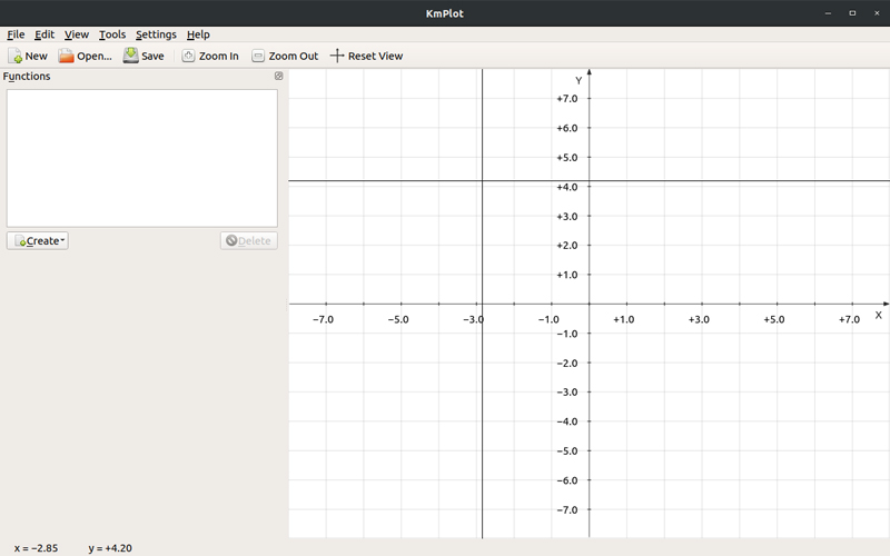
Figure 1. Upon start up, you can begin entering functions and learning about their behavior.

The first thing to do is create some functions to use from within KmPlot. Click the Create button at the bottom of the function window to bring up a drop-down menu. Here you can select from a number of plot types, such as Cartesian, polar or differential. As an example, clicking the Cartesian option opens a new window where you can create your function.

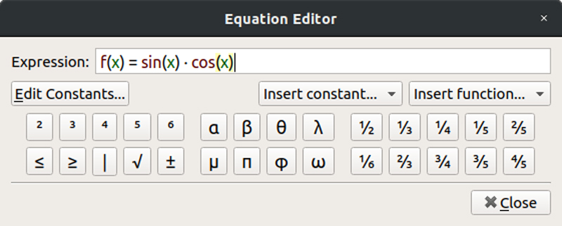
Figure 2. You can use the built-in palettes to select functions and constants to build up the functions that you are interested in.

You can use pre-defined constants and simpler functions to build up the specific function you want to study. Once you're finished, KmPlot will update the main window, and you'll see your plot generated.

Several defaults exist that you can assign in terms of its appearance. Click the Advanced button at the bottom of the left-hand pane to open a new dialog window where you can change some of the defaults.

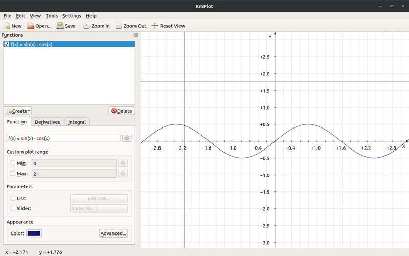
Figure 3. Click the Advanced button to set several options in the plot window.

Here, you can set the labels for the function name, as well as labels for the maxima and minima. The same lower left-hand pane also has tabs where you can get KmPlot to show the derivatives and integrals of the selected function. For example, you could plot the first derivative of a function.

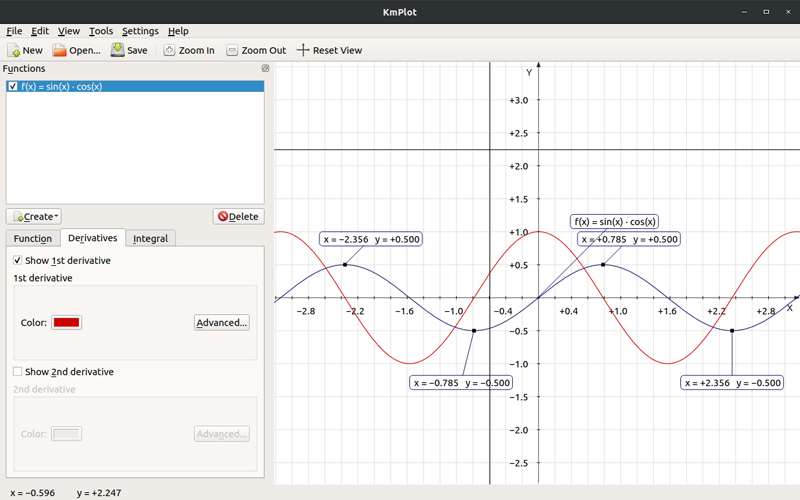
Figure 4. You can select to plot either the first or second derivatives of a given function.

To highlight the new plot better, click the color button and select a new color for the derivative curve. You also can plot the integral of a given function.

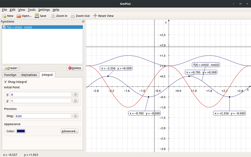
Figure 5. You can set several options for the integral, including the precision that the numerical method must reach when calculating and plotting the result.

You can create more complicated plots with combinations of functions. For example, you could plot both a regular Cartesian plot alongside a parametric plot.

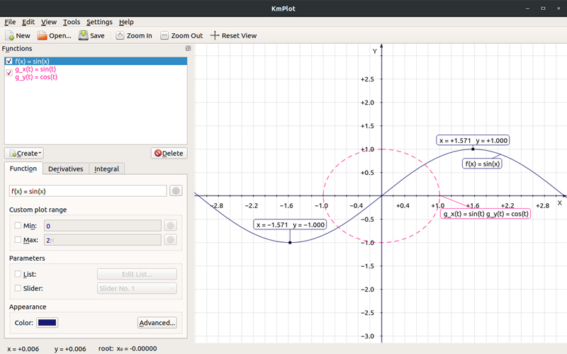
Figure 6. It sometimes helps to see multiple plots together to get better insight into the underlying mathematics.

This can be really useful when you want to gain a deeper understanding of a given function's underlying behavior. Looking at it from another angle, literally and figuratively, can be invaluable.

Several other tools also are available for working with these plots. Click Tools→Plot Area to open a new window where you can select one of the Cartesian plots and calculate the area between said curve and the x-axis. This is useful in physics and engineering contexts, where the area below a curve can have a physical analogue.

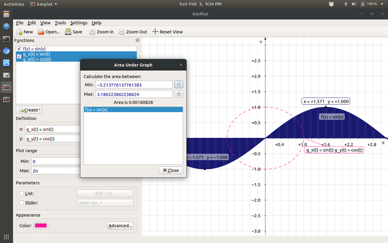
Figure 7. Sometimes you need to calculate the area below a curve, especially to get physical insights in a scientific context.

You also can click Tools→Calculator to open a new window where you can do quick calculations.

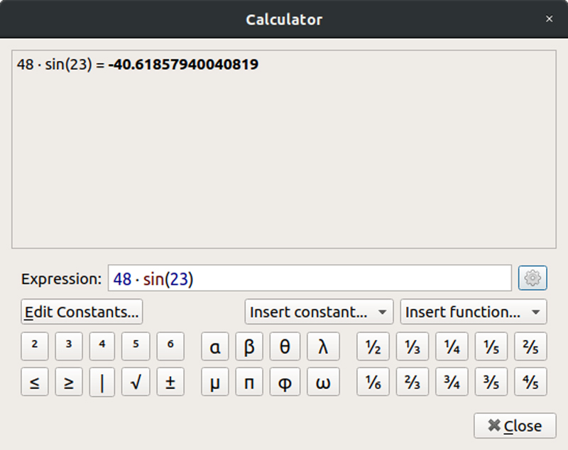
Figure 8. Sometimes you may need to make quick calculations while you are working on plots.

The last two items in the Tools menu are Find Maximum and Find Minimum. With these two options, you can ask KmPlot to find local maxima or minima. You just need to give it a range to search over, so that it can constrain the search.

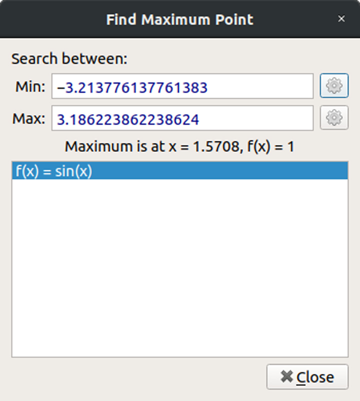
Figure 9. You can find the value of both maxima and minima for the functions that you are plotting.

You could have functions, such as the tangent function, which have a global maximum at plus infinity and a global minimum at negative infinity.

One of the most important parts of plotting a function is the coordinate system being used. In KmPlot, you can tailor the coordinate system by clicking View→Coordinate System. Here, you can change the x and y limits of the axes. As well, you can set the axis grid spacing. You can even define custom grid spacing functions.

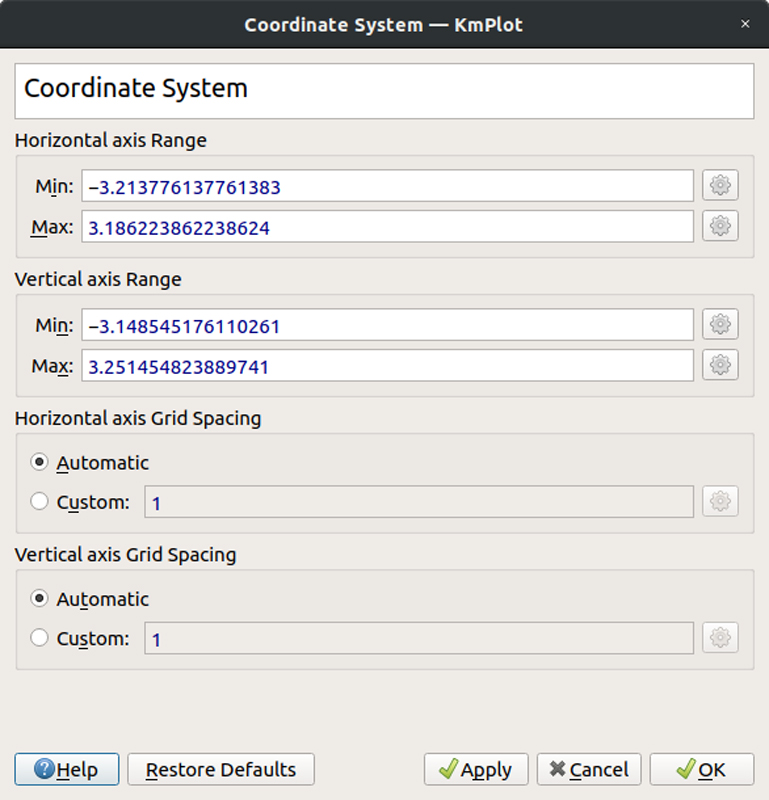
Figure 10. You can change several of the options of how the coordinate system is defined for the plots.

Because KmPlot is a part of the KDE project, it inherits several of that project's capabilities. One interesting ability is being able to script KmPlot's behavior. This is done through D-Bus commands. For example, you could tell KmPlot to plot a function with the following command:

You even can activate menu items and dialogs. You can use this functionality in order to include KmPlot as a component in a larger workbench or platform idea.

Once you have put some work into your analysis, you'll likely want to be able to save it. Click File→Save or File→Save As to save the work you have done in a proprietary file format. Another option for saving your work for other uses is to grab images of the plots themselves. Click File→Export to save the plot window in one of the usual image file formats. This way you can import them into documents or presentations.