
RTLinux meets one of the engineering world's most demanding control requirements, without requiring separate controller hardware and costing substantially less than comparable proprietary systems.
One of the most demanding applications of real-time control is the active magnetic bearing (AMB). Suspending a shaft rotating faster than 10,000 RPMs in a magnetic field with a gap of .015 inches—roughly the size of a grain of table salt—requires precise, reliable control of the magnetic field. Magnetic suspensions inherently are unstable. Think of a trapeze artist balancing a long pole on her chin, and you can appreciate the difficulty that a control system encounters when stabilizing a magnetic bearing. Magnetic bearings provide several advantages, however, which justify their use. The major advantage is magnetic bearings eliminate physical contact between the shaft and the support, minimizing friction and eliminating the wear inherent to conventional roller bearings.
A recent application under development in Japan is an implantable heart pump. Because magnetic bearings require no maintenance, this is an ideal situation in which to use them. For the same reason, satellite wheels also are a logical application.
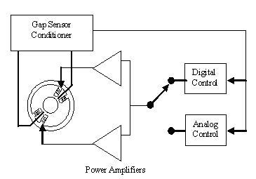
The experimental test rig, shown in Figure 1, consists of two eight-pole laminated stator assemblies, with individual windings on each of the poles. The bearing assembly includes inductive gap sensors at the centerline of each pair of diametrically opposed poles. These bearings support a two-foot-long shaft driven by a brushless DC motor. Figure 2 shows a schematic of a single axis. The controller uses the signal from the gap sensor to adjust the current from the power amplifiers driving the magnetic coils to keep the rotating shaft centered in the gap. The original controller was an analog circuit, which was replaced by the digital controller. The capability of running either the analog or digital controller is retained. The digital controller is implemented on an Intel Pentium III PC with a multichannel data acquisition board and a multichannel analog output board. The PC is configured as a dual-boot system, and the user selects plain Linux or RTLinux at startup.

Figure 2. Schematic of a Single Axis of the Magnetic Bearing
A real-time OS must ensure that a specific task executes at a fixed rate, regardless of the many system-level demands that burden the OS. To meet this requirement, two organizations, FSMLabs and RTAI, have developed special-purpose kernels that run Linux as a low-priority task within a real-time OS. This substantially reduces the timing from the hundreds of milliseconds on desktop systems to the microsecond range. It also allows the user to control precisely the timing of critical control processes.
For this magnetic bearing project, I selected the free RTLinux implementation from FSMLabs. RTLinux, developed by Michael Barabanov and Victor Yodaiken in 1996, currently is marketed by FSMLabs, a private company located in New Mexico. FSMLabs provides two versions of RTLinux, including RTLinux/Free, which I used for this project. FSMLabs holds a software patent on RTLinux, but the patent's license allows it to be used in projects licensed under the GNU GPL.
Conceptually, RTLinux splits the OS into user space and a real-time kernel. You may think of these as two separate cities, walled off from each other and able to communicate only by guarded pathways, such as real-time, first-in-first-out devices (RT-FIFOs). User space is the familiar Linux system with all its friendly utilities, such as the vi editor, the GCC compiler and the shutdown command. The real-time kernel is the Spartan environment that relentlessly executes the real-time task regardless of the activities in user space.
Real-time programs are coded as kernel modules and do not use the main{} program construct of user-space C programs. The module requires two functions: init_module, which is called when starting, and cleanup_module, which is called when turning off the real-time module. The init_module creates the entry point for the real-time module and allocates the RT-FIFOs used to communicate with user space. To start the real-time module, use the insmod command. Once the real-time module starts, it can be stopped only by issuing the rmmod command or by pulling the plug on the processor. As a new user of RTLinux, I was quite unnerved to discover that despite issuing the shutdown command, the controller continued to run.
Control theory, central to all modern technologies from the automobile to the jetliner, is an extensive field in which graduate students have toiled for many decades. I cannot cover this extensive body of theory here, but I can explain the essentials of the digital control for the magnetic bearing. First, the quantity to be controlled is instrumented and measured. In this case, the quantity is the gap between the rotating bearing and the magnetic poles of the bearing. This gap is converted to a voltage with signal conditioners and input to an analog/digital input (AI) board. In my setup, four separate gap sensor signals control the rotating shaft. All four gap signal voltages are sampled simultaneously.
The gap is controlled by the current traveling through the magnets, which are driven by eight power amplifiers. The power amplifiers are controlled by the voltage from a separate digital/analog output (AO) board. The AO board receives a digital input and converts it to a voltage that is held constant until the next signal. This sample-and-hold operation is fundamental to all digital control systems. In the control loop, the AO board receives the processed signals from the AI board after numerical processing. In an ideal digital controller, both AI and AO operations occur simultaneously at precise constant intervals. Although impossible to achieve this ideal, you must ensure that the code within the control algorithm runs efficiently. In my control program this occurs at 10kHz.
The numerical operations within the control program include the history of the input, x, and the output, y, of the controller for several previous steps. These are stored in memory and shifted one increment each time the control loop executes. The history is incorporated in a difference equation:
y(n)=A*y(n-1)+B*y(n-2)+...+C*x(n) + D*x(n-1) +...
where y(n) is the output of the controller for the current time step, y(n-1) is the output of the controller in the previous time step, y(n-2) is the output two steps in the past, y(n-3) is three steps in the past and so forth to the depth demanded by the sophistication of the control algorithm. Similarly, x(n) is the input voltage for the current time step, and x(n-1) is the input for the previous step. A, B, C, D and the rest are constant coefficients determined by the particular control law implementation. Controllers are either single-input-single-output (SISO) or multiple-input-multiple-output (MIMO). In my magnetic bearing test setup, y is the voltage driving the power amplifier, and x is the signal from the gap sensor. I use the three previous values in my magnetic bearing difference equation.
The digital controller is implemented on an Intel Pentium III PC operating at 1GHz with a six-slot PCI bus. The system was procured as a customized desktop personal computer with Red Hat Linux version 7.2 installed. In the laboratory the PC is not networked. I installed version 3.1 of RTLinux from a tar archive downloaded from FSMLabs.
The three possible approaches for selecting the digital acquisition and control (DAC) boards are to write the required board driver software, to obtain a driver from an open-source project such as Comedi and to use vendor-supplied driver software. The first and second options require a high level of sophistication and expertise with using Linux and data acquisition programming. The second option reflects the open-source nature of the Linux system, but the selection of vendors is limited and the latest products often are unavailable. The third option, although it requires the least expertise, places the user at the mercy of the board vendor. The vendors supplying and supporting the necessary drivers are limited and quite often use the same sources as the second option. In the end, I chose the third option and purchased two PCI bus multichannel DAC boards from United Electronics, Inc. These came with the required RTLinux drivers.
Before implementing the digital control law, I performed tests to characterize the digital system behavior. These tests are various program codes that evaluate conversion and timing interactions of the digital boards. For my primary functional test, I designed and coded a C language module that reads the analog data on the analog input board, converts it to floating point variables, converts it back to a digital variable and then outputs the signal by way of the analog output board.
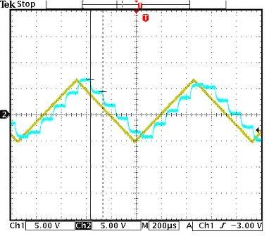
Listing 1 shows the skeleton of the C program for the primary functional test. At the heart of the real-time control program is the RTLinux function, pthread_wait_np, which suspends execution of the currently running real-time thread until the start of the next period. This thread is marked for execution using pthread_make_periodic_np. The thread gives up control until the next time period. The default arithmetic in RTLinux is integer. My control application requires floating point, which is turned on by pthread_setfp_np. A comparison of the input and output is recorded on a Tektronix two-channel digital storage oscilloscope. Figure 3 shows a typical record of system performance on this test. The main loop in the software is set at 10kHz in this plot; the analog input is a 1,000Hz sawtooth. The output shows the step waveform characteristic of sample-and-hold operation.

Figure 3. Oscilloscope Trace Showing Both the Test Signal (Yellow) and Analog Output (Blue)
A more intuitive way to test the operation of the system is to hook the analog output to an audio amplifier and speaker and input a sine wave from an external signal generator. I did this, and the tone was clean and steady. The original analog controller is a simple lead-lag filter on each of the four bearing axes, which is duplicated with the difference equation:
[ y(n) = 0.7467*y(n-1 )+ 4.6380*x(n) - 4.5189*x(n-1)]
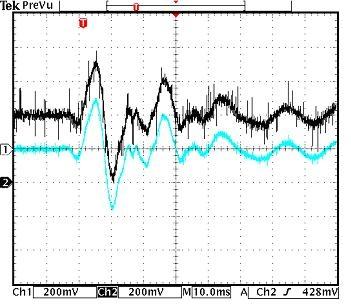
Figure 4 shows the digital and analog controller responses to a mechanical impulse on the shaft. The responses are virtually identical. In this figure, the digital controller response is shown at the top, and the analog controller response is at the bottom. The time shown in the figure is 100 milliseconds. The digital loop is operating at 10kHz in a MIMO configuration, which has five input channels and eight output channels.

Figure 4. Oscilloscope Trace Comparing Digital (Upper) to Analog (Lower) Controller Response to a Mechanical Impulse
Alternate control laws are implemented easily in C and experimentally verified. One of the more robust of these is shown in the difference equation:
y(n) = 1.4934*y(n-1) - 0.5576*y(n-2) + 0.5795*x(n) + .01487*x(n-1) - 0.5646* x(n-2)
The rotor has spun up to 11,000 RPMs successfully, with the AMB under full digital control, passing through a critical speed at 2,700 RPMs. In virtually all rotating machinery, from the humblest hair dryer to the modern passenger jet engine, critical speeds occur at distinct RPMs. At these critical speeds, the vibration of the rotating shaft grows large and places high loads on the bearings and other components. These present extreme tests for the bearings.
To change the coefficients of the control law while the rig is operating, I used RT-FIFOs. These are first-in-first-out files for communicating between Linux user space and RTLinux threads. Because RT-FIFOs are unidirectional, I created two separate files for two-way communication with the control module. Function rtf_create(fifo_id_no, fifo_length) allocates a buffer of the specified size for the specified FIFO ( /dev/rtf0, /dev/rtf1,..../dev/rtf64 ). It must be called from init_module(). Function rtf_destroy deallocates the FIFO at the completion of execution. It can be called from init_module( ) or clean-up_module(). This allows me to change the control law on the fly by changing the difference equation coefficients while the real-time module is running. Using the function rtf_get(fifo_id,&variables,sizeof(variables)) within the real-time thread reads the coefficients in a non-blocking mode. The user-space code for sending the coefficients to the real-time module is:
ctl = open("/dev/rtf1",O_WRONLY);
write(ctl,&coeffs,sizeof(coeffs));
ctl = close(ctl);
This code is embedded in an NCURSES interface, which allows me to change the coefficients with manual entries as the rig is rotating. The NCURSES Programming How-To by Pradeep Padala (see the on-line Resources) is an excellent resource for this work.
In a similar way, I can access the data stream in the control program and send it to user space. The appropriate function in the real-time module is rtf_put(framerate_rtfifo_id, volts, offset). In user space, send the output to a file with cat /dev/rtf0 > file . A simple C program to convert the file to a readable form must be written.
RTLinux is used to control a working rotor test rig at Tufts University. The controller is realized on a conventional Pentium III personal computer using the RTLinux extension of the Linux operating system. The control algorithm is implemented in C. Various control laws can be implemented and tried on an actual experiment.
An additional advantage is the elimination of a target computer, since the real-time OS operates on the same processor as the host computer. Most applications developed as digital control systems launch as a startup executable on a proprietary real-time target computer. The approach presented here differs; it does not target a RT controller based on a proprietary development system. It uses a Linux software environment developed for applications in control and data acquisition requiring hard real-time (deterministic) execution.
I wish to acknowledge the support of Professors Fred Nelson and Denis Fermental at Tufts for supporting this work. This work was partially funded by C. S. Draper Lab. of Cambridge, Massachusetts.
Resources for this article: /article/8260.